Nearest neighbor search
Nearest neighbor search is an optimization problem which involves finding a closest point (or k closest points) to a query q from a set of N points, based on a defined distance metric. It has numerous applications in fields such as computer graphics, machine learning (e.g., recommender systems, computer vision, classification) and information retrieval systems.
A naive approach to this problem is to calculate the distance from the point q to every point in our set of points. This brute-force search has a time complexity of O(n) and as our size of set grows, this algorithm becomes increasingly inefficient.
k-d Tree
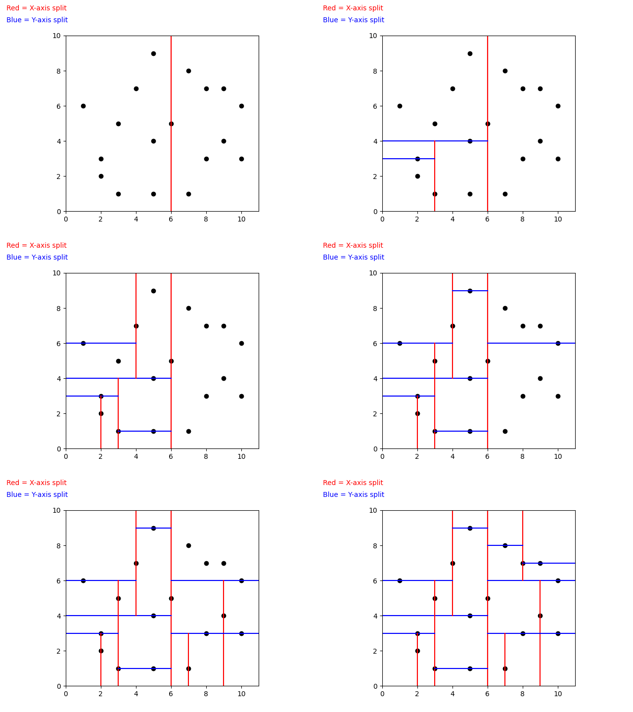
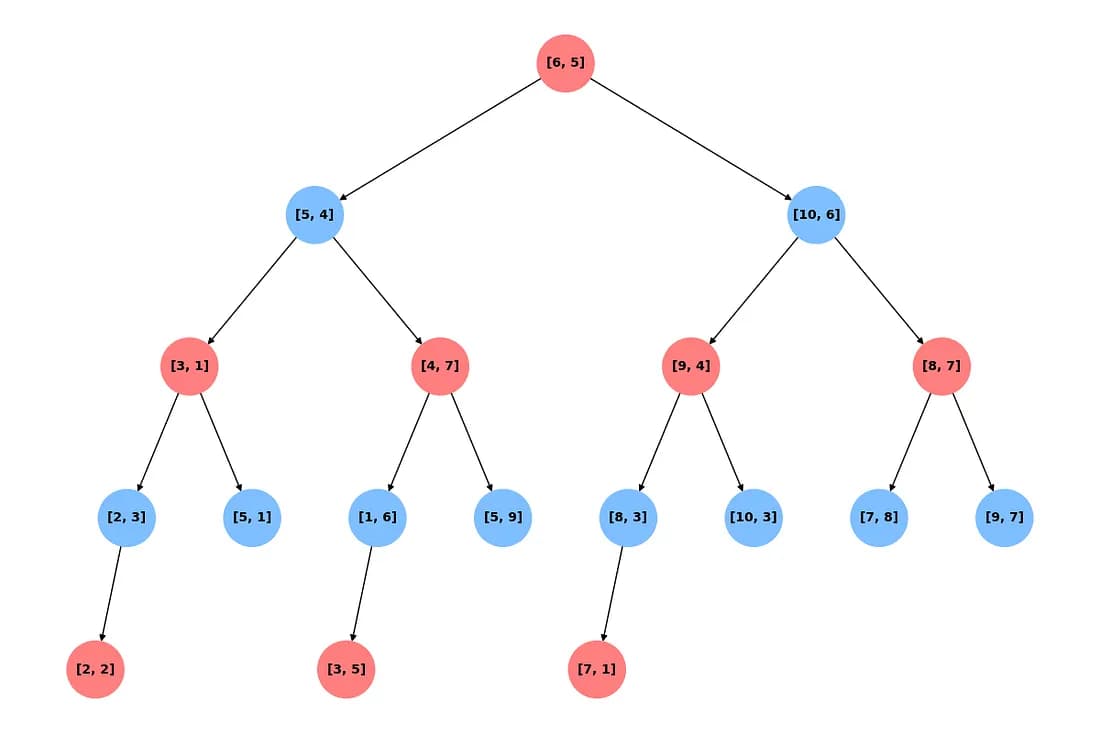
k-d Tree is a type of Binary Search Tree where every node represents a k-dimensional point and acts a splitting hyperplane that partitions the space into two regions along a specific axis. The left subtree contains points in one region, while the right subtree contains points in the other. For example, if an axis x is chosen as the splitting dimension, it would create a hyperplane perpendicular to the x-axis and all the points with values of x smaller, would go into the left sub-tree and all the points with greater values of x would go into the right sub-tree similar to a BST. k-d Trees typically use the Euclidean distance metric, which is inherently tied to their partitioning strategy and limits their applicability to other distance metrics.
Building a k-d Tree

When building a k-d Tree, pick a dimension for initial splitting. Ideally this should be the dimension with the highest variance in the data. This ensures that the data is divided more evenly. However, in practice, the data is often split in a fixed cyclic order.
splitting_dim = depth % k
#Or
next_splitting_dim = (current_splitting_dim + 1) % k
The data is split at the median point along the chosen dimension. We sort the points based on the splitting dimension, using algorithms like MergeSort or HeapSort which have a time complexity of O(nlog(n)). The median point is then added to the tree, and the process is repeated recursively with the points on the left (lower values) and right (higher values) of the median. This approach typically results in a fairly balanced k-d Tree.

Searching in a k-d Tree
When searching a k-d Tree, we start at the root node and compare the query point’s value along the splitting dimension with the current node’s value. If the query’s value at the splitting dimension is less than the current node’s value at the splitting dimension, we go the the left child and if its is greater, we go to the right child. We do it recursively, until we reach a leaf node. This is our approximate nearest neighbor and our current closest point.
However, it is possible that we have missed a point that is even closer. So we backtrack. It is possible that there is a point even closer than our current closest point if the distance from the query to the current splitting hyperplane is less than the distance to our current closest point. If this is the case, we also search in the other sub-tree to ensure we don’t overlook a closer point. The hyperplanes to which the distance is greater than our current closest point, we can safely prune the regions beyond them as they certainly cannot contain a closer point.
Curse of dimensionality
k-d Trees are efficient in low-dimensional spaces (around 10–20 dimensions). As the number of dimensions increases, the Euclidean distance metric looses its meaning as the data becomes sparse. And the space partitioning structure becomes less effective. Most of the points tend to be very close to the splitting hyper planes, resulting in increased number of backtracking and exploration of multiple sub-trees. In some cases its search time complexity can reach up to O(n), similar to a brute-force search.
Conclusion
In this article, we explored k-d Trees, focusing on how they are built and searched. It is an efficient space partitioning data structure that allows fast nearest neighbor search. However, their performance diminishes in high-dimensional spaces due to the curse of dimensionality.
